The monitoring question and reporting unit
This implementation guide considers Seasonal Baselines in the context of Seasonally dry forests, with Sentinel-1 Ground Range Detected backscatter as the selected data source. The purpose is to design a defensible monitoring workflow before purchasing imagery, selecting software settings or committing to an operational alert. Treat the proposed combination as a starting point for a feasibility assessment: the landscape may contain features that the product cannot resolve, and the relevant physical variable may differ from the decision a manager wants to make. Establish that relationship explicitly, then document what additional observations are required.
Landscape context and independent observations
Dry-forest monitoring must separate expected leaf shedding from persistent canopy disturbance. The relevant decision might concern clearing, post-fire recovery or unusual seasonal behavior. Define a forest and disturbance concept suited to the landscape, because sparse woody cover, shrubs and grass can coexist within the same satellite observation unit. Define the reporting unit, the observed variable and the action a finding could trigger before selecting an indicator. Retain these definitions so evaluation addresses the management question rather than visual appearance.
Rain onset and duration strongly affect leaf emergence and understory growth, while exposed soil becomes prominent during the dry season. Interannual rainfall variation can shift the apparent seasonal baseline. Compare similar phenological periods and retain rainfall context, instead of treating a greener wet year as evidence of permanent woody recovery. Record the observation window and comparison population. Consistent processing cannot compensate for dates or spatial units representing different processes. Preserve acquisition and context information so another analyst can reconstruct the comparison.
Grass flushes may create rapid greenness recovery after fire while woody structure remains damaged. Conversely, normal deciduous behavior can appear as extensive loss when dates are poorly matched. Bare ground, smoke and shadows can further confuse interpretation, so temporal persistence and independent evidence are essential before assigning a disturbance category. Treat competing explanations as hypotheses to test, with insufficient evidence retained as a legitimate result. Avoid forcing every difference into a problem class. Identify the additional observation that would change the interpretation.
Use reference sites covering woody cover, herbaceous cover and seasonal leaf states, with repeat observations where feasible. Deliver disturbance intervals and recovery indicators as separate layers. Explain whether each indicator tracks greenness, cover or structure, and avoid converting a seasonal spectral signal into biomass or biodiversity claims without suitable validation. Document reference selection and independence from threshold or model tuning. Preserve usable coverage and rejected observations. State the conclusion's spatial and temporal support so later updates remain comparable without overstating measured evidence.
Select the measurement and data product
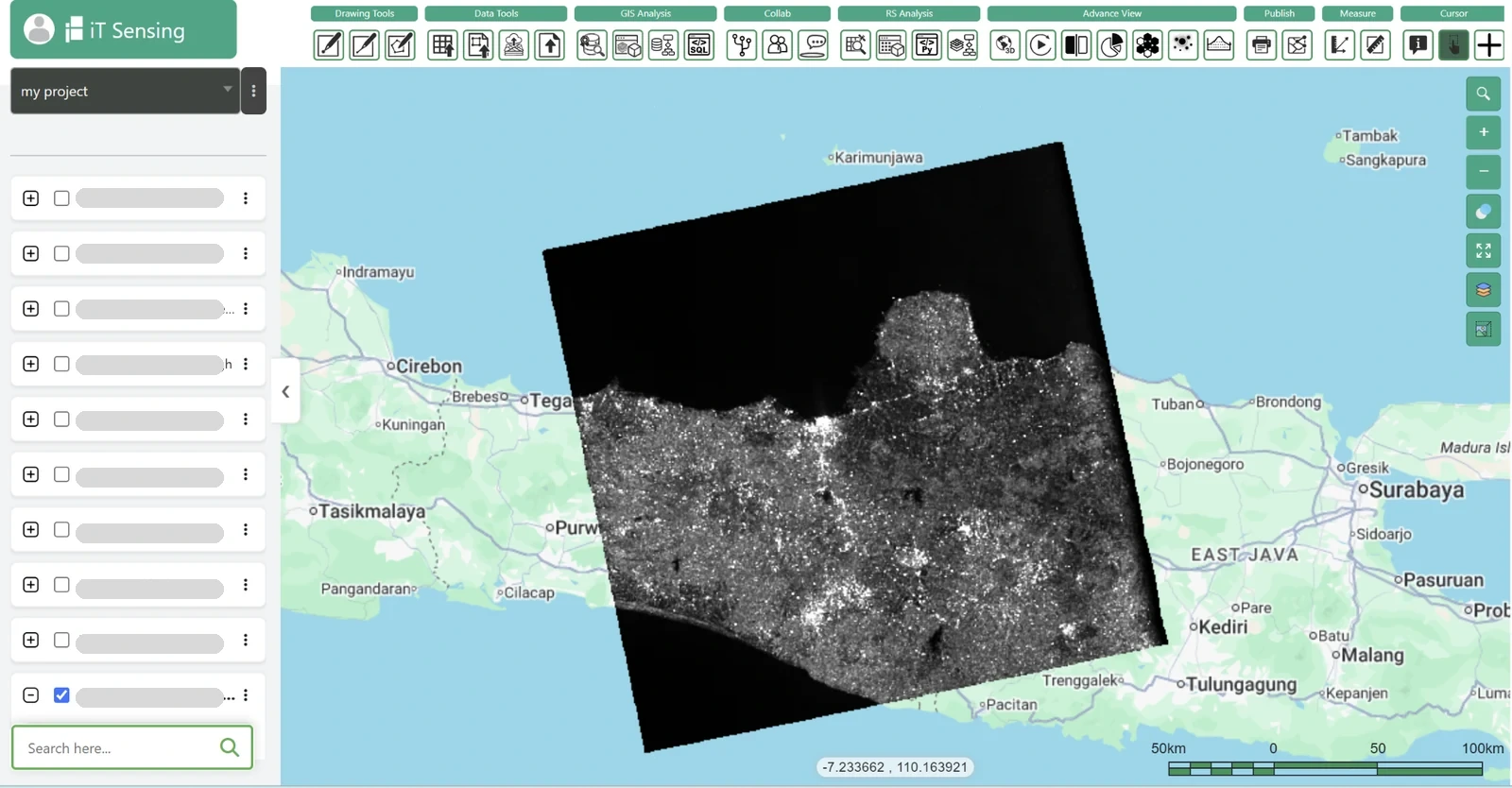
Sentinel-1 GRD represents detected radar intensity after processing that removes the complex phase information. C-band radar provides observations during darkness and through most cloud conditions, making it useful where optical coverage is limited. The signal responds to surface roughness, moisture, structure and viewing geometry. A darker pixel therefore cannot be assigned to water, damage or another class without checking the surrounding conditions.
Build a consistent series using matching acquisition mode, orbit direction, relative orbit and polarisation where practical. Radiometric calibration, terrain handling and noise treatment must be documented. State whether values are linear intensity or decibels before calculating averages and ratios. Speckle filtering can improve readability, but it also changes spatial support and can remove narrow features that matter to an operational analysis.
Terrain shadow and layover can make parts of a radar scene unsuitable for interpretation. Smooth dry surfaces may resemble open water, while flooded vegetation may produce stronger rather than weaker returns. Compare candidate changes with prior radar behaviour, terrain and independent observations. Keep an explicit unreliable-area mask, and do not describe radar access through clouds as universal ability to see every land-surface object.
Prepare and test the analysis
Define an expected condition before labeling a deviation as anomalous. A single previous image provides a change comparison, whereas a seasonal baseline describes the range of earlier comparable observations. Define the decision unit, observation period and consequence of an incorrect result before choosing processing settings. Separate the physical measurement from the management interpretation. The workflow should explain when available imagery is adequate, when more observations are needed, and who is responsible for reviewing uncertain cases.
Select comparable seasons, inspect long-term shifts and retain observation counts for each baseline interval. Exclude known invalid measurements without silently removing genuine extremes that are relevant to the decision. Keep a small representative test area and retain the original inputs. Record the product identifier, processing level, coordinate reference system and every setting that changes the numbers. Change one assumption at a time so that a reviewer can distinguish a processing effect from a real difference on the ground.
If hypothetical comparable historical values are 0.40, 0.42 and 0.44, their mean is 0.42. A current value of 0.30 is 0.12 lower; its significance requires more evidence. This is an illustrative calculation for checking the logic, not a measured outcome or a universal threshold. Repeat it on known inputs before processing the full region. Then vary the relevant assumption and document whether the decision changes, including cases where the available evidence cannot support a confident answer.
A changing sensor, land-management regime or climate can make old observations non-comparable. Short baselines also characterize variability poorly and can produce dramatic standardized anomalies from an unstable denominator. A plausible color pattern alone cannot resolve these competing explanations. Review representative failures alongside apparently successful locations, and compare observations made under similar conditions. Preserve a separate uncertainty or exclusion layer so that unsupported areas cannot quietly enter summaries as if they had the same evidential strength as reliable observations.
Test sensitivity to baseline years, seasonal window and minimum observation requirements. Check known stable and changed locations, and restrict interpretation where history is too sparse to establish expected variability. Set the acceptance rule before examining the final map. Use independent evidence that represents the difficult conditions as well as the easy ones. Report how many observations passed, which failed and why. A threshold that works in this test area still needs checking before transfer to another landscape or season.
Publish the baseline years, accepted observations, summary statistic and revision policy. Preserve the previous baseline when extending the historical archive so users can explain changes in reported anomalies. Package the analytical layer with its quality information and a short reproduction note. Include the acquisition dates, processing assumptions, limitations and responsible reviewer. Preserve stable identifiers across maps and tables so another analyst can trace a reported number back to its inputs and repeat the comparison without guessing the settings.
Interpret the combined evidence
Read the landscape and product sections together before applying the analysis procedure. In this guide, Seasonally dry forests defines the reporting context, while Sentinel-1 Ground Range Detected backscatter defines the available measurement; Seasonal Baselines supplies the processing and review question. These roles are deliberately separate. A working data connection does not establish that the measurement answers the management question. Reject a combination when the target is smaller than the effective observation scale, when the required season has no usable observations, or when the relevant property is not measured by the sensor. Retain that rejection in the project record so that an attractive demonstration does not become an unsupported operational promise.
Acceptance checks before delivery
Write acceptance conditions before inspecting the final map. Specify the reporting boundary, observation period, minimum valid coverage, reference sampling design and the consequence of an incorrect alert. Use project-specific values agreed with the recipient rather than copying a threshold from an unrelated landscape. Keep a small set of independent observations outside all parameter selection. Review omission and commission errors separately and examine boundary areas, rare conditions and missing dates. If the available reference observations do not cover the intended operating conditions, narrow the stated scope of the result instead of claiming that an apparently successful demonstration proves general reliability.
A useful GIS delivery contains more than a colored image. Export the analytical values where licensing permits, the validity mask, reporting geometries with stable identifiers, and a concise record of product names, acquisition dates, processing versions, coordinate reference system and resampling choices. Distinguish valid zero values from missing observations. Provide the area or count of usable measurements for every reporting unit and explain which units were excluded. A colleague should be able to trace a suspicious statistic back to the underlying observation without reconstructing the entire project from screenshots. Store the interpretation and its limits beside the data, not only in a presentation.
Connect the result with an ITSensing workflow
Use the ITSensing satellite catalog and remote sensing tools to evaluate the parts of this workflow that are available for the selected account and data source. Begin with a small representative area and compare the output with a trusted reference before scaling up. The product links below lead to the catalog, tools, documentation and plans so the team can check data access and processing requirements directly. This guide describes an analytical procedure; it does not assert that every named product, algorithm or export format is supplied natively by ITSensing. Where a step uses an external GIS or specialist tool, keep its inputs and outputs in the same reproducibility record.